Back to Kemp Acoustics Home


Next: Radiation impedance
Up: Multimodal propagation in acoustic
Previous: Projection along a cylinder
Contents
Method for calculation of pressure field
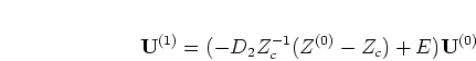
If we set  and
and  for
for  at the mouth of the horn, we have a
plane velocity at the input end of the horn. Physically this corresponds to
driving the input with a rigid piston. Using stored values of the impedance
along the guide we can project the volume velocity vector forward to the end
of the guide using the following equations:
at the mouth of the horn, we have a
plane velocity at the input end of the horn. Physically this corresponds to
driving the input with a rigid piston. Using stored values of the impedance
along the guide we can project the volume velocity vector forward to the end
of the guide using the following equations:
 |
(2.102) |
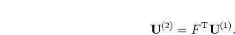
where  is a diagonal matrix with the
  th diagonal given by
 and
and  is a diagonal matrix with the th diagonal given
by
is a diagonal matrix with the th diagonal given
by  .
.
 |
(2.103) |
The pressure vector at each point along the horn is then given by
 .
.
The entries in the vector give the complex amplitude of each
mode. Consider the time dependence of the plane wave component of the
pressure at the input, having a complex amplitude  :
:
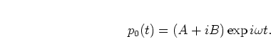 |
(2.104) |
This will have a maximum amplitude of
 and vary sinusoidally
in time:
and vary sinusoidally
in time:
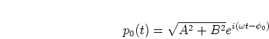 |
(2.105) |
where  is the angle of the pressure on the complex plane at
  :
:
 |
(2.106) |
Since the plane wave term in the volume velocity vector was chosen to be real
at the input end,
the volume velocity is at its maximum at and
the phase angle for the plane component of the
pressure vector at the input gives the phase angle by which the pressure
leads the volume velocity.
We will choose to plot the pressure field when
the pressure at the input is at its maximum. From
equation (2.105)
we see that this occurs at time
 .
.
Now consider the pressure at some point along the length of the duct where
the complex pressure amplitude of the th mode is  :
:
 |
(2.107) |
Putting
and taking the real part gives the physically
observable pressure field when the plane pressure is maximum at the input:
 |
(2.108) |
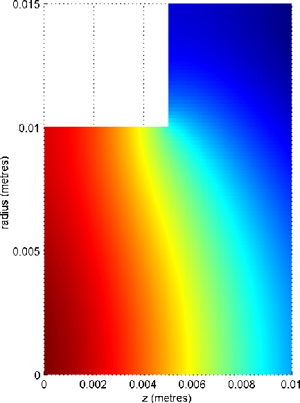
Figure 2.9 shows the pressure field calculated in this
manner for a cylinder of length 5mm and radius  mm driven by a piston
vibrating sinusoidally at 10 kHz connected to
a cylinder of radius
mm driven by a piston
vibrating sinusoidally at 10 kHz connected to
a cylinder of radius  mm assuming lossy propagation.
25 modes were used and the system was approximated by 1000 cylinders for
the calculation. The termination on the right is the
infinite cylindrical pipe termination
mm assuming lossy propagation.
25 modes were used and the system was approximated by 1000 cylinders for
the calculation. The termination on the right is the
infinite cylindrical pipe termination
 where
where  .
Here red indicates the maximum value of the real part of the pressure
and blue the minimum.
.
Here red indicates the maximum value of the real part of the pressure
and blue the minimum.
Notice that the wavefronts expand out from the opening. The contours of
equal pressure are perpendicular to the walls as required by the hard walled
boundary condition. The pressure is continuous at the discontinuity showing
that the algorithm correctly projects the modes across.
Figure 2.9:
Pressure field of a piston driven cylinder terminated in an infinite cylindrical pipe
 |
Back to Kemp Acoustics Home
Next: Radiation impedance
Up: Multimodal propagation in acoustic
Previous: Projection along a cylinder
Contents
Jonathan Kemp
2003-03-24