Acoustic pulse reflectometry measurement with MLS excitation

It is important to realise at this stage that the system impulse response, $h$, of a reflectometer is not simply the input impulse response of the object on the output end of the reflectometer; it includes the impulse response of the loudspeaker, the losses in the source tube, the input pulse passing the microphone on its way to the loudspeaker, the source reflections and so on. The system impulse response, $h$, that we have calculated can be chopped to isolate the object reflections. These object reflections are equivalent to those that can be measured by the conventional pulse excitation except that our signal to noise ratio is much improved. The deconvolution of object reflection and calibration pulse measurements is still necessary when using MLS excitation.

MLS signals are inherently periodic with a period of $2^m-1$. In equation (7.8) the system impulse response, $h$, (which is not periodic) is convolved with the MLS signal, $s$. The result is that $y$ is the periodic response of the system to continuous excitation by the periodic MLS. When we perform our experiments, we must choose an MLS signal whose period time is larger than the total response time of the system in order to prevent the end of our calculation of the system response folding back onto the start. Similarly, we must play the MLS signal end to end twice and ignore the response during the first run through in order to make sure that the response we are measuring conforms to the periodicity condition.

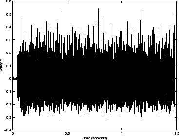
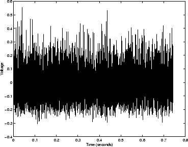
Figure 7.11 shows the signal recorded at the microphone when an MLS signal of order $m=15$ is fed into the loudspeaker. The shorter reflectometer with $l_1 = 7.37$m and $l_2 = 3.10$m is used and data acquisition is performed in Matlab for Windows with a Guillemot soundcard at a sample rate of $F_s=44100$Hz. Sampling of the microphone reflections is started and then the start of the MLS signal is fed to the loudspeaker. The signal from the loudspeaker should take $l_1/c = 7.37/343 \approx 0.02$s to reach the microphone. In fact, the first 0.04 seconds of the recording consists only of undesired background noise, showing that there is delay of 0.02 seconds between the start of the sampling and the start of the MLS signal leaving the loudspeaker. This delay is caused by computer processing time and means that care must be taken when we are isolating the part of the system impulse response corresponding to the object reflections or calibration pulse.

The time period for a $m=15$ sequence is $(2^m-1)/F_s = 0.743$ s which will also be the time length of our resulting measurement data for the system impulse response. This is considerably longer than the total time taken for an acoustic pulse to decay to zero as can be deduced from the fact that the pressure waves are much reduced by losses and reflection from the loudspeaker after 0.1 seconds in say figure 7.3. As mentioned previously, both the MLS and measured response are assumed to be periodic by the theory. Figure 7.11 shows the microphone pressure sampled while two periods of the MLS are played by the loudspeaker, end to end. The microphone signal during the second period therefore features the response to the last part of the previous period of excitation so satisfying the periodicity requirement. This signal is shown isolated in figure 7.12.

Figure 7.11: Microphone signal for excitation with a $m=15$ MLS signal repeated twice

Figure 7.12: Microphone signal chopped to show one period of response to continuous excitation with a $m=15$ MLS signal

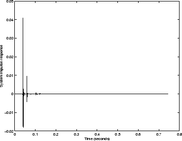
The auto-correlation of the MLS input and the recorded response from figure 7.12 was performed in the frequency domain using equation (7.14). Figure 7.13 shows the result. This is the full system impulse response and features the input pulse passing the microphone, the reflection of the pulse from the closed end of the source tube and the source reflections. The response shows that all acoustic energy decays to zero about 0.2 seconds after a pulse is produced as was expected.

Figure 7.13: System impulse response

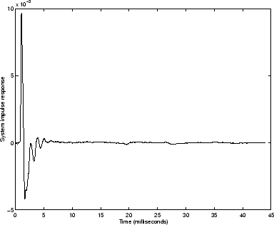
Figure 7.14 shows the calibration pulse or reflections from the closed end of the source tube obtained by chopping the system impulse response. The exact recorded time at which the calibration pulse arrives in the system impulse response depends on the time lag between the starting of sampling and the starting of the excitation as mentioned previously. This time lag depends on the software, hardware specifications and the computational load. In order to avoid this problem, the sample in the system impulse response with the maximum value (corresponding to the maximum of the input pulse) is first found. The position of the reflections from the closed end or test object can be defined relative to this point, meaning that the input/output time lag does not effect the results. This experiment can be repeated with a musical instrument or test object on the end of the source tube and analysed with the calibration pulse measurement to obtain the bore reconstruction and input impedance. By selecting appropriate delay times, the virtual dc tube and source reflection cancellation methods can be used.

Figure 7.14: Calibration pulse isolated from system impulse response

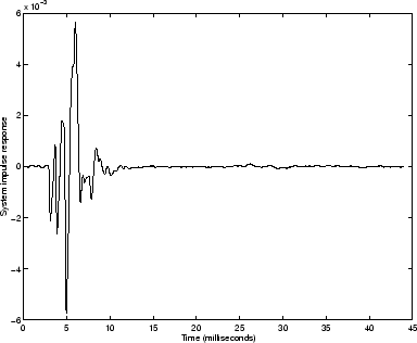
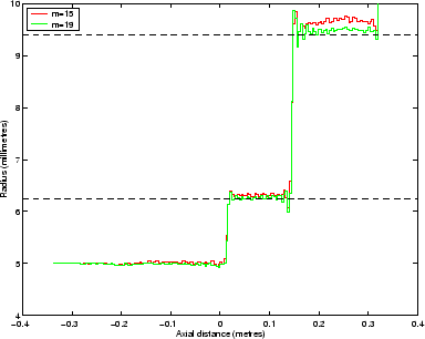
Figure 7.15 shows the object reflections obtained by chopping a system impulse response measurement performed with the short stepped cylinder test object used in chapter 5 on the end of the source tube. As with the previous experiment an MLS of order $m=15$ was used. The object reflections were isolated from the system impulse response 2ms earlier than for the calibration pulse, meaning that the virtual dc tube method can be applied.

Figure 7.15: Object reflections isolated from system impulse response

Figure 7.16 shows the resulting bore reconstruction with $m=15$. Also shown is the result of performing the experiment with excitation with a much longer MLS signal of $m=19$. Such an MLS signal will have a time length of $(2^m-1)/F_s = 11.89$ s. Calculating the discrete Fourier transform of a signal this length takes several seconds with the current computational power available. Using an increased order means that more energy is added to the system, so improving the signal to noise ratio. The bore reconstruction with $m=15$ measures the radius of the final cylindrical section to be 0.4 mm too large, while the $m=19$ measurement is much improved, averaging just 0.1 mm more than the correct value. The level of oscillations in supposedly cylindrical sections of bore are slightly reduced by the increase in order. This implies that the noise level at high frequency is reduced by the fact that we have added more energy to the system. The fact that the $m=19$ reconstruction of the last cylinder has an average value closer to the correct radius is evidence of greater accuracy at low frequencies.

Figure 7.16: Reconstructions for different orders of MLS excitation