Back to Kemp Acoustics Home


Next: Solutions for a uniform
Up: Solutions for a cylinder
Previous: Loss-less propagation
Contents
So far we have discussed the behaviour of acoustic waves in tubes assuming
that none of the acoustic energy is lost to heat. In reality there is a
boundary layer immediately beside the tube walls in which viscous and thermal
losses occur.
It is possible to use a lossy boundary condition to give lossy versions of
 and
and  but the
effect of losses will be noticeable in the
but the
effect of losses will be noticeable in the  direction only because
we will be considering objects which are significantly longer than they are
wide. The inclusion
or exclusion of the effect of losses will therefore be represented entirely
by the choice of direction wavenumber,
direction only because
we will be considering objects which are significantly longer than they are
wide. The inclusion
or exclusion of the effect of losses will therefore be represented entirely
by the choice of direction wavenumber,  .
Starting with a lossy boundary condition which allows a small
acoustic particle velocity flow into the wall of the tube, Bruneau et al
[44] have produced a complex direction wavenumber:
.
Starting with a lossy boundary condition which allows a small
acoustic particle velocity flow into the wall of the tube, Bruneau et al
[44] have produced a complex direction wavenumber:
![\begin{displaymath}
k_n =
\pm \sqrt{k^2 - \left(\frac{\gamma_n}{R}\right)^2
...
...R}\right)
[ \mbox{Im}(\epsilon_n)-i \mbox{Re}(\epsilon_n) ]}
\end{displaymath}](img182.png) |
(2.53) |
where  is the boundary specific admittance at the wall.
Admittance is the reciprocal of the impedance, so gives a measure of the
acoustic velocity into the wall for a given acoustic pressure. The
implication is not that there is really a flow into the walls
(which are rigid in reality) but that the loss of energy at the
boundary layer is simulated by imagining that such a flow exists.
The boundary specific admittance is given by [44]:
is the boundary specific admittance at the wall.
Admittance is the reciprocal of the impedance, so gives a measure of the
acoustic velocity into the wall for a given acoustic pressure. The
implication is not that there is really a flow into the walls
(which are rigid in reality) but that the loss of energy at the
boundary layer is simulated by imagining that such a flow exists.
The boundary specific admittance is given by [44]:
 |
(2.54) |
with
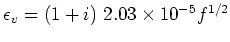 and
and
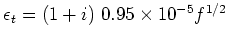 under standard
conditions. The full expressions for
under standard
conditions. The full expressions for  and
and  in terms of
the thermodynamic constants of air are given in [44].
in terms of
the thermodynamic constants of air are given in [44].
The choice of signs is complicated by the fact that we are performing the
square root operation on a complex number. To split into real and
imaginary parts, it is helpful to first express (2.53) as follows
 |
(2.55) |
where  is the square of in the absence of losses:
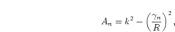 |
(2.56) |
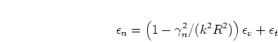
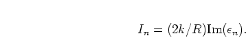
 gives the imaginary part of the correction in
  :
:
 |
(2.57) |
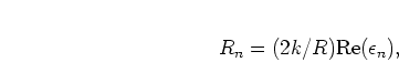
and  is the real part of the correction in :
 |
(2.58) |
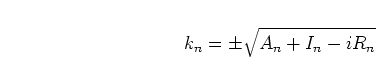
Now we can express in terms of real and imaginary parts:
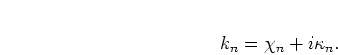 |
(2.59) |
Equating equations (2.55) and (2.59) we get
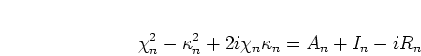 |
(2.60) |
which can be solved by simultaneous equations for the real and imaginary parts
giving [44]
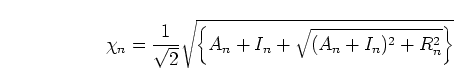 |
(2.61) |
and
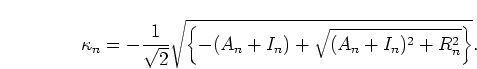 |
(2.62) |
Putting  this equation gives the imaginary part of the
plane mode wavenumber as
this equation gives the imaginary part of the
plane mode wavenumber as
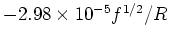 .
.
Back to Kemp Acoustics Home
Next: Solutions for a uniform
Up: Solutions for a cylinder
Previous: Loss-less propagation
Contents
Jonathan Kemp
2003-03-24