Back to Kemp Acoustics Home


Next: Lossy propagation
Up: Solutions for a cylinder
Previous: Solutions for a cylinder
Contents
Assuming axi-symmetric pressure distributions only,
equation (2.31) becomes:
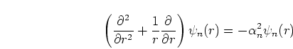 |
(2.44) |
which can be manipulated into Bessel's equation of order zero
[43] with the general solution ([43] p567)
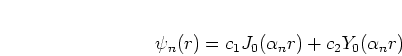 |
(2.45) |
where  is Bessel function of the first kind of order zero and
  is
the Bessel function of the second kind of order zero. While is singular
at the origin, the pressure cannot have a singularity there.
All the physically realisable solutions will therefore have
is
the Bessel function of the second kind of order zero. While is singular
at the origin, the pressure cannot have a singularity there.
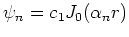
All the physically realisable solutions will therefore have  .
The pressure on a cross-section on the
.
The pressure on a cross-section on the  -
- plane will therefore follow
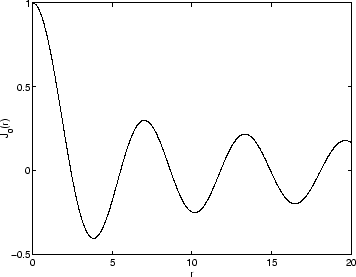
the shape of the Bessel function . A three dimensional plot of
is shown in figure 2.4 while figure 2.5 shows the function
along the radial direction. It has a maximum at
plane will therefore follow
the shape of the Bessel function . A three dimensional plot of
is shown in figure 2.4 while figure 2.5 shows the function
along the radial direction. It has a maximum at  and smoothly
varies between positive and negative values. The rate at which this happens
for
and smoothly
varies between positive and negative values. The rate at which this happens
for
 is determined by the - plane
wavenumber,
is determined by the - plane
wavenumber,  . In order to work out the allowed values of ,
we must consider the boundary conditions.
. In order to work out the allowed values of ,
we must consider the boundary conditions.
Figure 2.4:
Three dimensional plot of the Bessel function of the first kind of order 0 against radius on the - plane
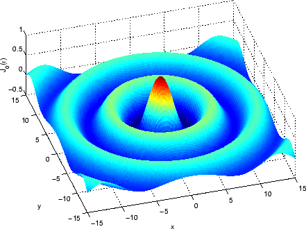 |
Figure 2.5:
The Bessel function of the first kind of order 0
 |
The boundary condition for loss-less propagation is
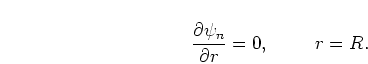 |
(2.46) |
Using the orthogonality relation (as used by Kergomard [42])
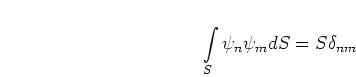 |
(2.47) |
we get the solution
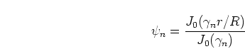 |
(2.48) |
where  are the successive zeros of the derivative of the Bessel
function of order zero. From relation (A.3) in
Appendix A we see that the derivative of is
are the successive zeros of the derivative of the Bessel
function of order zero. From relation (A.3) in
Appendix A we see that the derivative of is
 . is therefore also equal to the zeros of the Bessel
function of order one. These are tabulated for
. is therefore also equal to the zeros of the Bessel
function of order one. These are tabulated for  to
to  in
Appendix A. The corresponding values of are then:
in
Appendix A. The corresponding values of are then:
 |
(2.49) |
Recalling equation (2.32) the  direction wavenumber is
given in terms of the - plane wavenumber and the free space wavenumber
as
direction wavenumber is
given in terms of the - plane wavenumber and the free space wavenumber
as
 |
(2.50) |
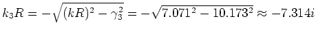
For  the square root
is of a positive number and the positive sign should be taken in
equation (2.50) so that
the square root
is of a positive number and the positive sign should be taken in
equation (2.50) so that  is a positive real wavenumber. For
 , however, the square root is of a negative number
and the mode will have an imaginary wavenumber in the direction.
Provided the negative sign is chosen in equation (2.50), the
direction pressure profile of that mode will then be
, however, the square root is of a negative number
and the mode will have an imaginary wavenumber in the direction.
Provided the negative sign is chosen in equation (2.50), the
direction pressure profile of that mode will then be
 |
(2.51) |
which shows exponential damping. The modes of a duct will therefore
propagate provided the wavenumber (and therefore frequency) is above the
cut-off frequency
 and will be exponentially damped
otherwise. To summarise, the signs are chosen to be
and will be exponentially damped
otherwise. To summarise, the signs are chosen to be
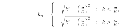 |
(2.52) |
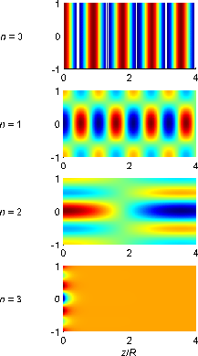
Figure 2.6 displays a false colour image of the forward travelling
modes in a cylinder (note one mode is in cut-off so is not really travelling).
The horizontal axis runs parallel to the axis of the cylinder ()
while the vertical axis runs perpendicular to the axis of the cylinder such
that the value 0 is the centre of the cylinder and -1 and 1 are the walls.
To obtain the pressure distribution along the axis of the cylinder
equation (2.52) was substituted into equation
(2.33). This was multiplied by the transverse
eigenfunction from equation (2.48) to give the
full pressure field.
The real value of the complex pressure amplitude was chosen so
that a snapshot of the pressure field is shown, rather than a time averaged
value, as would be the case if the absolute value was shown. The relationship
between the complex pressure amplitude and the time dependence of the pressure
field will be discussed in more detail later, in section 2.7.
Red indicates the pressure maximum and blue the pressure minimum in each graph.
Figure 2.6 shows plane wave propagation ( =0) for a
wavenumber of
=0) for a
wavenumber of
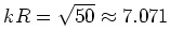 .
The =1 mode with the same free space
wavenumber is also shown. Notice that the pressure distribution follows the
Bessel function profile across a line perpendicular
to the cylinder axis. Since the modes we are considering are cylindrically
symmetric the two nodal lines parallel to the axis for =1 become one
nodal
cylinder when this image is considered in 3 dimensions. The whole distribution
varies sinusoidally along the axis with the wavenumber . Notice that
.
The =1 mode with the same free space
wavenumber is also shown. Notice that the pressure distribution follows the
Bessel function profile across a line perpendicular
to the cylinder axis. Since the modes we are considering are cylindrically
symmetric the two nodal lines parallel to the axis for =1 become one
nodal
cylinder when this image is considered in 3 dimensions. The whole distribution
varies sinusoidally along the axis with the wavenumber . Notice that
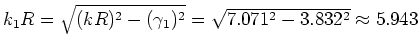 so the direction
wavenumber has decreased and therefore the direction wavelength has
increased. This effect can be seen more clearly with the =2
mode. The pressure distribution has two nodal cylinders and we can see that
so the direction
wavenumber has decreased and therefore the direction wavelength has
increased. This effect can be seen more clearly with the =2
mode. The pressure distribution has two nodal cylinders and we can see that
 is approaching zero for this choice of free space wavenumber:
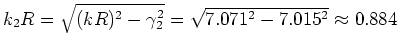 .
The
.
The  value is below the cut-off point,
  in the case of the
=3 mode.
in the case of the
=3 mode.
 meaning that the wave is
exponentially damped or evanescent.
meaning that the wave is
exponentially damped or evanescent.
Figure 2.6:
The modes in a cylindrical duct with (plane wave mode),  ,
,  and
and  (evanescent). All have the same free space wavenumber
 |
Back to Kemp Acoustics Home
Next: Lossy propagation
Up: Solutions for a cylinder
Previous: Solutions for a cylinder
Contents
Jonathan Kemp
2003-03-24