Multimodal equations at a discontinuity

So far we have provided the equations describing the behaviour of the modes of uniform ducts with circular and rectangular cross-section. As mentioned before, the aim of this chapter is to enable the calculation of acoustic variables in a duct of varying cross-section. The method employed here is to discretise the smoothly varying duct into a large number of concentric cylinders (or rectangles). While we have already seen equations which describe propagation within each cylinder, we still need to analyse how the modes of the duct are effected by changes of cross-section. This section deals with this problem.

Consider again the typical discontinuous join between two sections of tube of differing cross-section shown in figure 2.2. The pressure field at either side of the discontinuity must be equal on the section of air they share. However, the $n$th mode on $S_1$ will not match the $n$th mode on $S_2$ because the cross-sections are different. This means that when the $n$th mode is incident on the discontinuity, the pressure on the other side must consist of the sum of the contributions of many modes. We say that the wave experiences mode conversion at the discontinuity.

Now this will be put into our mathematical framework. We recall ${\mathbf P}^{(1)}$ is the vector of modal pressure amplitudes on the surface $S_1$ and define ${\mathbf P}^{(2)}$ as the vector of modal pressure amplitudes on the surface $S_2$. In circular cross-section, when $R_2>R_1$, ${\mathbf P}^{(1)}$ can be found from ${\mathbf P}^{(2)}$ by projection. This procedure can also be performed in rectangular geometry when $a_2>a_1$ and $b_2>b_1$.

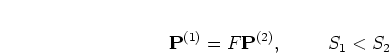
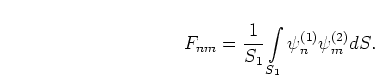
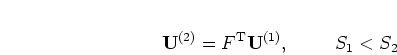
The following expression relating the pressure vectors on either side of the discontinuity is derived in appendix B using the orthogonality of Bessel functions:

$${\mathbf P}^{(1)}= F {\mathbf P}^{(2)}, \mbox{\hspace{1cm}} S_1 < S_2$$ (2.79)

where $F$ is a matrix with the elements defined by

$$F_{nm} = \frac{1}{S_1}\int\limits_{S_1}\psi_{n}^{(1)}\psi_{m}^{(2)}dS.$$ (2.80)

When $R_1>R_2$ or $a_1>a_2$ and $b_1>b_2$, the pressure must be equated on the smaller $S_2$ surface. This means that the equations look the same but with the labels 1 and 2 interchanged:

$${\mathbf P}^{(2)}= V {\mathbf P}^{(1)}, \mbox{\hspace{1cm}} S_1 > S_2$$ (2.81)

where $V$ is a matrix with the elements defined by

$$V_{nm} = \frac{1}{S_2}\int\limits_{S_2}\psi_{n}^{(2)}\psi_{m}^{(1)}dS.$$ (2.82)

The integration in equation (2.80) will be performed analytically to get the elements of the matrix $F$. The expression for the elements of the matrix $V$ will follow from the derivation by symmetry. Note that to avoid unnecessary complication we will not treat rectangular ducts which contract along the $x$ direction while at the same time expanding along the $y$ direction or vice versa.

The vector $\mathbf{U}$ can be projected by equating the axial velocity on the air shared by $S_1$ and $S_2$. Also the axial velocity is required to be zero into the wall surface perpendicular to the $z$ axis which results from $S_1$ not equalling $S_2$. For $S_1<S_2$ the axial velocity on either side is therefore matched on $S_1$ and set to zero on the part of $S_2$ which is not in contact with $S_1$. 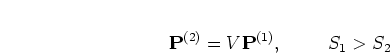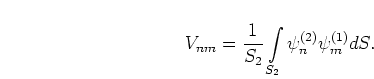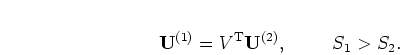The calculation is performed in detail in appendix B to give

$${\mathbf U}^{(2)}= F^{\mathrm{T}} {\mathbf U}^{(1)}, \mbox{\hspace{1cm}} S_1 < S_2$$ (2.83)

where $F^{\mathrm{T}}$ is the transpose of $F$. For $S_1>S_2$ the axial velocity is therefore equated over $S_2$ and set to zero on the part of $S_1$ not in contact with $S_2$.

$${\mathbf U}^{(1)}= V^{\mathrm{T}} {\mathbf U}^{(2)}, \mbox{\hspace{1cm}} S_1 > S_2.$$ (2.84)