Back to Kemp Acoustics Home


Next: Results
Up: Multimodal radiation impedance of
Previous: Multimodal radiation impedance of
Contents
Analysis
Expressing (3.13) in cylindrical coordinates for a cylindrical duct
of radius  :
:
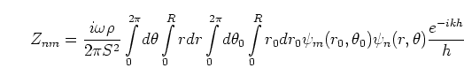 |
(3.14) |
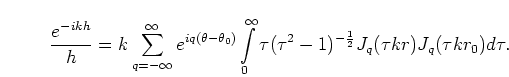
where
![\begin{displaymath}
h = [r^2 + r_0^2 - 2rr_0 \cos(\theta-\theta_0)]^{\frac{1}{2}}.
\end{displaymath}](img331.png) |
(3.15) |
As discussed in section 2.4.1, we will be treating
cylindrically symmetric modes only.
From equation (2.48), the mode profile on the surface is
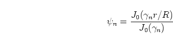 |
(3.16) |
where  is the
  th zero of the Bessel function
  and is
tabulated in appendix A.
and is
tabulated in appendix A.
Now we will give  in terms of
  , a dummy variable of
integration. We will show that all the other variables of integration will
then have an analytic solution. Sonine's integral from Watson [52]
p.416 gives:
, a dummy variable of
integration. We will show that all the other variables of integration will
then have an analytic solution. Sonine's integral from Watson [52]
p.416 gives:
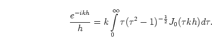 |
(3.17) |
The integrand is imaginary when  and real when
  .
Care must be taken when choosing the sign of
.
Care must be taken when choosing the sign of
 with the negative and imaginary interpretation taken here when .
Notice that we have been using the
opposite sign convention from Zorumski [37] for the imaginary part
throughout because we are assuming a time factor
of
with the negative and imaginary interpretation taken here when .
Notice that we have been using the
opposite sign convention from Zorumski [37] for the imaginary part
throughout because we are assuming a time factor
of
 rather than
 .
.
Neumann's addition formula [52] p.358 is
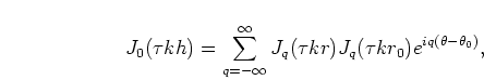 |
(3.18) |
which can be substituted into (3.17) to give
 |
(3.19) |
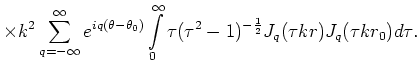
Now substituting (3.19) into (3.14) we get
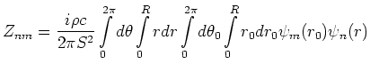 |
|
|
|
 |
|
|
(3.20) |
Note that
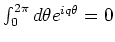 unless
  , in which
case it is equal to
, in which
case it is equal to  .
Integrating by
.
Integrating by  and
and  then gives a factor of
  .
When rearranged, the integral can be reduced to
.
When rearranged, the integral can be reduced to
 |
|
|
(3.21) |
where
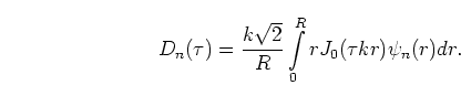 |
(3.22) |
The integration in equation (3.22) can be found analytically
(see equation (A.1) in appendix A):
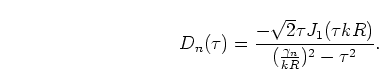 |
(3.23) |
The four dimensional integral has now been reduced to a one dimensional
integration, with the variable  (and therefore the singularity mentioned at
the end of section 3.3.1) eliminated.
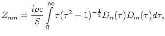
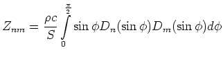
Noticing that in equation (3.21) the integral is real for
(and therefore the singularity mentioned at
the end of section 3.3.1) eliminated.
Noticing that in equation (3.21) the integral is real for
 and imaginary for
  , we split the integral into real
and imaginary parts with variables
, we split the integral into real
and imaginary parts with variables
 and
and
 respectively.
 |
|
|
|
 |
|
|
(3.24) |
Now
 and
and
 .
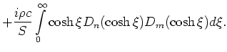
Remembering that the negative imaginary interpretation should be
taken for the resulting
.
Remembering that the negative imaginary interpretation should be
taken for the resulting
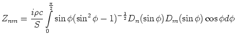
 we get
 |
|
|
|
 |
|
|
(3.25) |
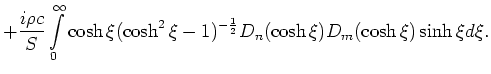
The first integral can be performed by numerical integration using
Simpson's rule or an equivalent.
In the second integral, however, the range extends to infinity.
The integrand is an oscillatory function of  whose amplitude of
oscillation decays exponentially to
whose amplitude of
oscillation decays exponentially to  typically at around
  .
Numerical integration can then be performed from 0 and 10 without
incurring any significant numerical errors.
.
Numerical integration can then be performed from 0 and 10 without
incurring any significant numerical errors.
Back to Kemp Acoustics Home
Next: Results
Up: Multimodal radiation impedance of
Previous: Multimodal radiation impedance of
Contents
Jonathan Kemp
2003-03-24