Results for a trumpet section

The next step is to calculate the input impedance of an object to give an example of the convergence of the calculation. We chose to perform the calculation on a bore which matches that of the bell section of a standard trumpet. The section was obtained by simply cutting the instrument in two after the valve section and 50.4 cm before the open end of the bell. Physical measurement of the bore was performed using calipers and the results are listed in table 4.1. In order to perform the multimodal calculation, we need to know the radius at any point along the bore, not just at the measured points. This was obtained by 3rd order polynomial interpolation using the two nearest data points on each side of the place of interest.

Table 4.1: Trumpet section dimensions

$z$ (cm)	0	0.2	0.7	7.0	11.02	11.87	16.21	20.73	25.0
$R$ (mm)	6.8	6.5	6.5	6.5	6.5	6.72	7.32	8.25	9.12
$z$ (cm)	29.7	34.5	36.9	39.0	42.5	45.4	48.2	49.7	50.4
$R$ (mm)	10.07	11.7	12.7	13.7	16.2	19.8	32.7	47.5	64.5

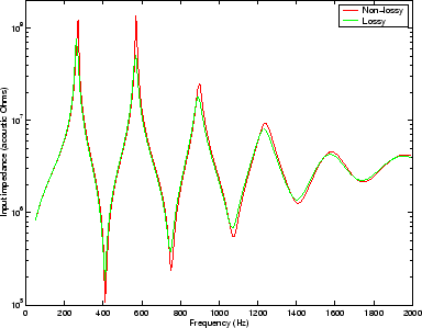
A calculation of the input impedance of the trumpet section was performed using the lossy wavenumber given in section 2.4.1 and using the non-lossy wavenumber of equation (4.8). The first 11 modes were included in the calculation and the horn was approximated by 1000 cylinders, each of length 0.504 mm. Figure 4.2 shows the absolute value of the input impedance for these calculations.

Inclusion of losses is observed to decrease the strength of resonance behaviour in the instrument. The height and frequency of the peaks in the input impedance are reduced. This is characteristic of loss of energy; less pressure is built up for the same excitation velocity at resonance. The depth of the troughs are reduced at impedance minima when losses are included because the reflections which return from the open end of the instrument are less strong, so decreasing the destructive interference responsible for anti-resonance.

Figure 4.2: Trumpet section input impedance

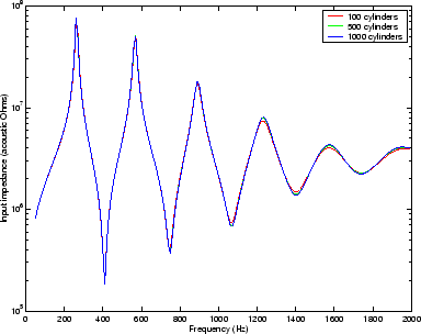
Figure 4.3 shows the absolute value of the input impedance of the trumpet section calculated with the first 11 modes included and the lossy wavenumber used. The calculation was performed by approximating the horn by 100 cylinders of length 5.04 mm, then the calculation was repeated using 500 cylinders of length 1.008 mm and 1000 cylinders of length 0.504 mm.

The results are very similar, showing that the input impedance calculation is not sensitive to the exact step size chosen. The 500 and 1000 cylinder calculations show convergence to an accuracy of $2\%$. This accuracy is good enough for this type of calculation because peaks and troughs differ by several orders of magnitude, as can be seen from the logarithmic scale.

Figure 4.3: Trumpet section input impedance

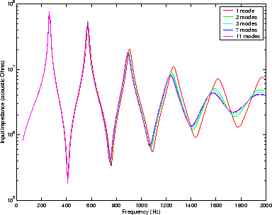
Figure 4.4 shows how the calculation of the absolute value of the input impedance of the trumpet section (approximated by 1000 cylinders with the lossy wavenumber used) varies with number of modes included. Results are shown when the vectors and matrices in the calculation are truncated to 1 mode (which gives a plane wave calculation), 2, 3, 7 and 11 modes. The 7 and 11 mode calculations show convergence to $2\%$ indicating that the inclusion of more modes in the calculation would have no significant effect.

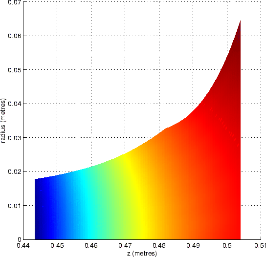
It is worth noting the cut-off frequency of the second mode (first non-planar mode) at the bell. Here the radius is maximum at $R=6.45$ cm and so the cut-off frequency is at its minimum at $f_c = k_c c/(2 \pi) \approx 3.83\times 343/(0.0645\times 2\pi) \approx 3240$ Hz. All modes except the plane mode are in cut-off (ie. are strongly evanescent) at all points along the trumpet in the frequency range of interest. The input impedance of the first five or so modes clearly still has an effect on the input impedance due to mode coupling. Including extra modes has a similar qualitative effect to the inclusion of viscothermal losses. The frequency and height of the impedance peaks are reduced at resonance while the anti-resonance behaviour is less marked because of the energy lost due to coupling with evanescent modes.

Figure 4.4: Trumpet section input impedance

The impedance matrix was stored at each step along the guide for the 580 Hz excitation, and this information was used to calculate the complex pressure amplitude vector at each step using the method described in section 2.7. Figure 4.5 shows the resulting pressure field when the calculation is truncated to 1, 2, 3, 5 and 11 modes. The frequency 580Hz is just above the second resonance peak. At the input, the phase angle is $\phi_0=-1.06 = -0.337 \pi$ radians which indicates that the volume velocity is leading the pressure. This is characteristic of a tube playing above resonance [2]. Results not presented here for frequencies just below resonance show a very similar pressure field but with the pressure leading the velocity at the input.

Red indicates a global maximum pressure and blue a global minimum pressure while the black lines are equipotential contours. All graphs show the same qualitative pressure along the axis of the horn. There are two pressure anti-nodes along the axis of the horn because we are close to the second resonance frequency of the horn. The first is a pressure maximum at the input end indicated by the red colour. The second anti-node is 180 degrees out of phase with the first and so gives a negative pressure peak (ie. global pressure minimum) at this point in the resonance cycle. It is visible as the dark blue colour 27 cm down the horn. The are two pressure nodes. The first is where the acoustic pressure crosses zero around 15 cm down the horn. The other is where the acoustic pressure approaches zero at the bell. These are represented by a mid-range colour, turquoise.

The plane mode calculation has flat pressure wavefronts as expected. The 2 mode calculation allows the pressure on a cross-section to be the sum of the plane wave and the $n = 2$ mode pressure distribution which has a maximum in the middle, one nodal circle and a local maximum at the edge. The resulting pressure map therefore shows non-planar pressure wavefronts. As more modes are added, the pressure field converges to show wavefronts meeting the wall at 90 degrees as required by the hard walled boundary condition. Notice that the radius and $z$ scales are the same, as required to prevent distortion of the angle at which the equipressure contours meet the wall.

Figure 4.5: Trumpet section pressure field: (a) plane wave approximation, (b) 2 modes, (c) 3 modes, (d) 5 modes, (e) 11 modes

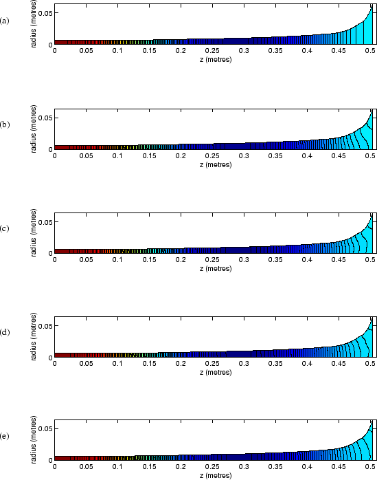Figure 4.6 shows a close up of the 11 mode pressure field at the bell. Here the equipressure contours can be seen as stripes of uniform colour, without the aid of black lines. Notice that the colour map has been changed in that the full range of colours are used for an area of bore which was previously all the same colour. The node at the bell has an acoustic pressure of approximately zero while the nearest anti-node on the left has negative acoustic pressure. The node at the bell is therefore the maximum pressure on the graph and is represented by red. The increasingly negative acoustic pressures on the left then give the minimum pressures present, represented by dark blue.

Figure 4.6: Trumpet section pressure field: 11 modes