In sections 6.3 and 6.4 we performed multimodal scattering from a discontinuity for an example in which there was no backward going wave on the right hand side. In order to create the multimodal version of our scattering equation (6.17), we must drop this assumption and express the pressure and volume velocity as the sum of forward and backward going waves on both sides. The aim then is to start with the known forward going and backward going waves at the input to a discontinuity (ie. from an experimentally measured input impulse response), and calculate the forward and backward going waves on the other side of the discontinuity. This method was suggested by van Walstijn [60].
We will denote the forward going pressures on surface 1 and surface 2
respectively as
![]() and
and
![]() .
The backward going pressure on surface 1 and surface 2
respectively will be
.
The backward going pressure on surface 1 and surface 2
respectively will be
![]() and
and
![]() .
Again the surfaces are as shown in figure 5.1.
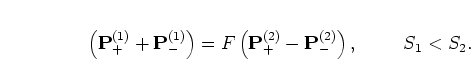
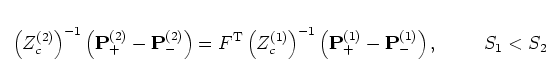
Using the pressure projection equation (2.79) we get:
.
Again the surfaces are as shown in figure 5.1.
Using the pressure projection equation (2.79) we get:
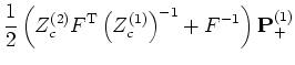
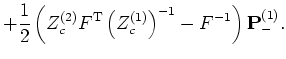
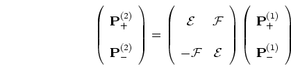
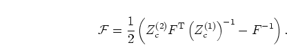
It is possible to express both equations (6.22) and (6.23) in
one equation. This is done by making column vectors consisting of the
forward going and backward going pressure vectors end to end. If the vectors
![]() and
and
![]() are each
truncated to have
are each
truncated to have ![]() elements, the resulting end to end vector will
have a length of
elements, the resulting end to end vector will
have a length of ![]() elements. This is then set equal to a single scattering
matrix with
elements. This is then set equal to a single scattering
matrix with ![]() elements multiplied by a vector of length
elements multiplied by a vector of length ![]() consisting of the pressure vectors
consisting of the pressure vectors
![]() and
and
![]() placed end to end.
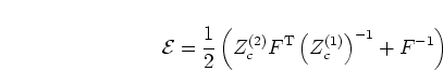
The first
placed end to end.
The first ![]() columns
in our scattering matrix then come from the coefficients of
columns
in our scattering matrix then come from the coefficients of
![]() in the previous equations and the second
in the previous equations and the second ![]() columns
from the coefficients for
columns
from the coefficients for
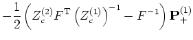
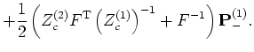
![]() . The resulting equation is
. The resulting equation is
 |
(6.25) |
 |
(6.26) |
Each of the elements in equation (6.24) is frequency dependent so we must compute the scattering matrix for each frequency in the Fourier transform of the pressure signals and perform the matrix multiplication in the frequency domain. This method means a significant increase in the computational load. Only a small number of modes could be added for this method of bore reconstruction to be feasible.
In addition to scattering across discontinuities, scattering along cylindrical sections is also necessary. We will therefore require multimodal versions of equations (6.18) and (6.19) which give the pressure value at surface 3 from the pressure value at surface 2 in figure 5.1. The modes propagate independently between these surfaces because the cross-section remains constant. For a given frequency of sound, the wavelength along the axis of the duct depends on the mode under consideration, with higher order modes having longer wavelengths untill at high enough mode numbers the waves are exponentially damped. This means the pressure is not just delayed by travel along the pipe, it also experiences dispersion.
The dispersion is described in the time domain by Morse and Ingard
[22] p.498. Firstly, below cut-off the ![]() modes are exponentially
damped meaning that the low frequencies are filtered out.
Above cut-off, the phase velocity is larger than
modes are exponentially
damped meaning that the low frequencies are filtered out.
Above cut-off, the phase velocity is larger than ![]() and the group velocity
is smaller than
and the group velocity
is smaller than ![]() , with both converging on
, with both converging on ![]() in the high frequency limit.
The time domain impulse transfer function for a higher mode pressure
distribution is calculated by Fourier transform to give
an impulse travelling at the speed of sound
in the high frequency limit.
The time domain impulse transfer function for a higher mode pressure
distribution is calculated by Fourier transform to give
an impulse travelling at the speed of sound ![]() with a wake trailing behind.
Physically this is realistic since an impulse contains all frequency
components, with the very high frequencies responsible for the sharp impulse
travelling with a group velocity of
with a wake trailing behind.
Physically this is realistic since an impulse contains all frequency
components, with the very high frequencies responsible for the sharp impulse
travelling with a group velocity of ![]() and the lower frequency components
following behind.
and the lower frequency components
following behind.
Using this impulse transfer function for time domain
convolution with the forward and backward going pressure vectors is a possible
solution for scattering down a cylindrical section.
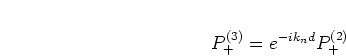
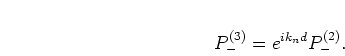
Alternatively, frequency domain multiplication can be
used. The pressure amplitude of the ![]() th higher mode in a uniform pipe is
described in equation (2.33). Projecting the forward
going part gives
th higher mode in a uniform pipe is
described in equation (2.33). Projecting the forward
going part gives
 |
(6.27) |
 |
(6.28) |